GIS II: Raster Modeling

Goals and Objectives

The purpose of this lab was to gain experience using various raster geoprocessing tools to build sand mining suitability and sand mining impact models.  These models took both environmental and cultural risks into account within the study area of Trempealeau County, WI.  

Methods

Frac Sand Mining Suitability Model 

Figure 1: suitability index model

During the first part of this lab, I utilized specified criteria and raster geoprocessing tools to create a suitability index model in ArcGIS (Figure 1).  For each criterion, I determined class breaks and suitability ranks, using the following scale: 3 = High, 2 = Moderate, 1 = Low.  My justifications for my rankings can be found in Figure 2.

The following criteria was used to calculate mining suitability: 

• Geology
• Land Use & Land Cover
• Distance to Railroads
• Slope
• Water Table Depth

Figure 2: suitability ranking justification table

Frac Sand Mining Impact Model 

Figure 3: impact index model

During the second part of this lab, I utilized specified criteria and raster geoprocessing tools to create a impact index model in ArcGIS (Figure 3).  For each criterion, I determined class breaks and suitability ranks, using the following scale: 3 = High, 2 = Moderate, 1 = Low.  My justifications for my rankings can be found in Figure 4.

The following criteria was used to calculate mining impact: 

• Streams*
• Prime Farmland
• Residential Areas
• Schools
• Wildlife Areas

*For streams, I decided to only use Order 2 - 9 (Strahler Stream Order) streams since contamination of larger streams poses a greater risk to surrounding environments.  

Figure 4: impact ranking justification table

Overlay of Models 

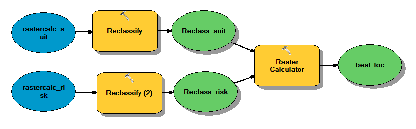
Figure 5: best locations model

After creating both a suitability and impact index model, I overlaid these two models using Raster Calculator to ascertain the best locations for frac sand mines in Trempealeau County, WI (Figure 5).  

Viewshed 

Finally, to gain some experience using the Viewshed Tool in Arc Map, I chose to take a look at visibility from a few parks in Trempealeau County, WI. This was a valuable exercise since the Viewshed Tool can be very useful within the fields of military geography and urban planning, among others. 

Results

After running all of my models, I utilized ArcMap to create cartographically pleasing maps depicting my findings. 

Frac Sand Mining Suitability Model 

Figure 6: suitability maps

Frac Sand Mining Impact Model 

Figure 7: impact maps

Best Locations

Figure 8: best location map

Viewshed

Figure 9: viewshed tool map

Discussion

After examining my map detailing the best locations for frac sand mines in Trempealeau County, I determined that the northwestern corner of the county seemed to have both the best suitability and least risk (Figure 8).  It is important to remember, however, that only ten factors were assessed during this lab.  Countless other factors such as commerical areas, major roadways or locations of current mines could influence the final placement of a mine.  Additionally, in-person site inspections should be carried out to make final determinations since models are not completely reliable.  Despite this, my models and final map provide a valuable, albeit general, look at the best locations for sand mines.  

Conclusions

This lab demonstrated that raster geoprocessing tools can be very effective for analysis purposes.  Through utilizing a systematic and logical ranking system, I was able to create useful suitability and impact models, which, when overlaid, produced a best locations map.  I really enjoyed completing this lab since it served as a synthesis of all of the work we have done this semester.  

Sources

Cropland Cover. In United States Department of Agriculture. Retrieved March 15, 2016 from http://datagateway.nrcs.usda.gov/

Trempealeau County Land Records. Retrieved March 15, 2016 from http://www.tremplocounty.com/tchome/landrecords/

United States Department of Transportation. Retrieved March 15, 2016 from http://www.rita.dot.gov/bts/sites/rita.dot.gov.bts/files/publications/national_transportation_atlas_database/index.html

United States Geological Survey. Retrieved March 15, 2016 from http://nationalmap.gov/about.html

Web Soil Survey. In United States Department of Agriculture. Retrieved March 15, 2016 from http://websoilsurvey.sc.egov.usda.gov/App/HomePage.htm

GIS II: Network Analysis

Goals & Objectives

The goal of this lab was to perform network analysis in order to calculate the impact of frac sand trucking on local roads as a part of our semester-long GIS II project.  

Background: 
Before beginning this lab, I completed some background reading to inform myself on the effects of fracking truck transportation upon local communities by reading the white paper "Transportation Impacts of Frac Sand Mining in the MAFC Region: Chippewa County Case Study."  As the text explains, frac sand mines are often located in remote areas in the country, which means that many of the resources used for the mining process (water, sand, chemicals, drilling equipment) need to be transported to and from the mining site.  This transportation has adverse effects upon local roads, which has caused local governments to explore ways to mitigate this damage.  Chippewa County, for example, has developed a series of road upgrade maintenance agreements (RUMA) to deal with recovering road damages, funding maintenance, and grading cross improvements (Figure 1).  

It is important for counties to be aware of the level of heavy truck traffic so they are able to plan accordingly for repairs.  Different types of sand mining operations have different transportation impacts as well, all of which require varying levels of cost and mitigation efforts (Figure 2).  Wisconsin legislation states that counties must be reimbursed for damage incurred on county highways, so knowledge and tracking of damages can be financially beneficial to county governments.  

Figure 1: list outlining aspects of a quality RUMA (white paper)

Figure 2: table detailing impacts of different frac mining operations (white paper)

Methods

At the beginning of this lab, I wrote a Python script (view here under Python Script #2) to select the mines to be used in my network analysis.  This script selected mines that were: 

• active
• did not have a rail loading station
• not within 1.5 kilometers of a railroad

After this, I utilized Model Builder in ArcMap to create a model (Figure 3) that achieved these objectives: 

• determined to which rail terminal each mine should travel
• determined the most efficient route from each mine to a rail terminal
• determined the length of each route (and cumulative lengths within each WI county)
• estimated hypothetical costs that each route/county would incur

To achieve the first two objectives, I utilized the Make Closest Facility Layer tool to specify a route from each mine to a rail terminal.  Then, I projected these routes as well as my counties feature class to a Wisconsin projection.  After this, I used the Tabulate Intersection tool to carry out an intersection between the routes and counties boundaries feature classes.  Then, I added two new fields to the resulting table, namely a Roads Length and a Costs field.  In the first, I used Field Calculator to calculate the total length of roads affected by trucks in each county.  In the second newly created field, I used hypothetical values to calculate a cost estimate.  In this hypothetical scenario, I assumed that each mine had 50 trucks travel to the rail terminal and back again, with it costing 2.2 cents per truck per mile. It is important to note that these values are purely hypothetical and do not represent actual transportation costs by any means.  The final attribute table displayed route lengths and estimated costs by county (Figure 4).    

Figure 3: network analysis model in ArcMap

Results & Discussion

The results of my methods can be seen below (Figure 4, Figure 5).  The table and map clearly display the scope of frac sand mine trucking and its effects, which are especially prevalent in Chippewa County, Eau Claire County and Barron County.  It is interesting to consider these routes after reading the aforementioned white paper; each county government has a say in how these routes and roads are used and maintained by frac sand mine trucks.  In Chippewa County, RUMAs are implemented to ensure that roads are kept up and frac sand mine companies are held accountable for the damage they incur on the roads.  Such results could prove useful to county governments in negotiating compensation from frac sand mining companies.  

Figure 4: output table from model displaying road length & cost by county

Figure 5: final map showing truck routes

Conclusions

Prior to completing this lab, I had primarily only considered the negative effects that frac sand mining has upon humans and the environment.  This lab, however, caused me to think about the ethics involved in fracking.  Public roads are free to be used by everyone, but when certain vehicles' intensive use causes damages, should they be held accountable?  According to Wisconsin law and my own convictions, yes.  The process behind calculating the effects of such damage and the monetary compensation required can be done via network analysis in ArcMap.  

Sources

National Center for Freight and Infrastructure Research and Education. (2013). Transportation Impacts of Frac Sand Mining in the MAFC Region: Chippewa County Case Study.  Retrieved from http://midamericafreight.org/wp-content/uploads/FracSandWhitePaperDRAFT.pdf 

Network Dataset analysis performed using data from ESRI Street Map USA.

GIS II: Data Normalization, Geocoding, and Error Assessment

Goals & Objectives

The aim of this lab was to gain experience in normalizing raw data, geocoding addresses, and conducting error analysis.  As this lab is an extension of the GIS II semester-long frack sand mine project, the study area was on Trempeleau County and nearby counties in western WI.  Data used in this lab was provided by the WI DNR.  

Methods

This lab involved multiple phases, as detailed by Figure 1.  

Figure 1: work flow of geocoding process

Normalization

Firstly, I normalized the raw data which was provided by the WI DNR in an Excel table (Figure 2).  The normalization process involved separating PLSS descriptions from street addresses, as well as placing other information into the appropriate columns.  After finishing this, the table was ready to be imported into ArcMap (Figure 3).  

Geocoding

Next, I used the geocoding service provided through ArcGIS Online to geocode my mines.  Since some mines had street addresses, some had PLSS descriptions, and some had both, I used two different techniques to locate the mines.  

I first took a look at all of the addresses that had been automatically geocoded by ArcGIS to see if the locations seemed accurate.  For the mines that had street addresses given by the WI DNR, the automatically geocoded locations were often nearby the actual locations. If the given address seemed inaccurate, I utilized Google Maps and/or the WI DNR website's map of frack sand mines to try to identify the correct location.  Then, upon finding a likely location, I manually selected the address.  

If a mine only had a PLSS description and no street address, the automatically geocoded location was always incorrect and needed to be manually located.  To do this, I imported PLSS base data including townships, sections and quarter-sections.  Then, I was able to identify the mines and manually select the correct address.  

Error Analysis

After geocoding all of my frack sand mine locations, I compared my geocoded locations to my classmates' and the actual mine locations.  This process involved using the "Near" tool in ArcMap and creating a map and error table to display the differences in locations (Figure 4 and Figure 5.  

Results

Normalization

Figure 2: raw data provided by the WI DNR

Figure 3: normalized data ready for import into ArcMap

Geocoding & Error Analysis

Figure 4: map depicting geocoded locations

Figure 5: table displaying differences in geocoding results;
"null" denotes that no other locations existed for comparison

Discussion

Though most of my geocoded locations were more or less accurate, elements of error were also present, as seen by Figure 4 and Figure 5.  The three locations that were most inaccurate (from the actual locations) were mines 209, 210 and 305.  Using Lo's chapter entitled "Data Quality and Data Standards," I took a look at the reasons behind these errors. 

Error in the first two sites, 209 and 210, could be explained by attribute data input error due to inherent causes.  The addresses were 125 19 1/4 St. and  2559 5 1/4 Ave., both comprised of multiple numbers which could have easily been slightly jumbled (i.e. 125 19 1/4 St vs. 1251 9 1/4 St.) during initial input by the WI DNR.  Furthermore, this error could be explained as feature classification or coding error as a result of operational causes--ultimately a gross error.  Since both 209 and 210 were inactive mine sites, they were more difficult to identify and could have led to human blunder when geocoding.  

Error in site 305 is most likely the result of human blunder and is best classified as gross error.  This site only had a PLSS description and not a street address provided, so I had to utilize PLSS base data to try to locate the mine.  I found this process much more difficult since only a general location was provided, not a street.  

Ultimately, we can know which locations are actually correct by using the latitude and longitude data provided by the WI DNR.  This data is the most accurate data on-hand, though some gross error could have occurred during the DNR's data collection process in the field. 

Figure 6: error table (Lo, Chapter 4)

Conclusion

Through this lab, I learned the intracacies of the complicated process known as geocoding.  Though geocoding is an important aspect of spatial analysis, it is important to be wary of inherent and operational errors that may occur and affect your final outcomes.  I think that a better result could have been achieved in this lab if we had worked with the other five people who were geocoding our same mines to develop more consistency in methods.   

Sources

Wisconsin Department of Natural Resources. Retrieved April 4th, 2016 from http://dnr.wi.gov

Lo, CP. (2003). Concepts and Techniques in Geographics Systems. Retrieved April 4th, 2016.

GIS II Lab 2: Data Downloading, Interoperability, and Working with Projections in Python

Goals & Objectives

This lab concerned locating, downloading and organizing spatial data.  The study area was Trempealeau County, WI, which pertains to our semester-long GIS II project regarding frack sand mining.  

Specific goals addressed in this lab include increasing proficiency in: 

• downloading data from the internet
• data organization
• importing data to ArcGIS
• joining data
• projecting data from different sources into one coordinate system
• building and designing a geodatabase
• basic Python scripting
• determining data accuracy

Methods

The first section of this lab dealt with data management.  First, I downloaded data about Trempealeau County from six different online sources using the workflow depicted in Figure 1. 

Figure 1: work flow of data management

These sources included:

1. US Department of Transportation
2. USGS National Map Viewer
3. Multi-Resolution Land Characteristic Consortium
4. USDA Geospatial Data Gateway
5. Trempealeau County Land Records
6. USDA NRCS Web Soil Survey

After the data was appropriately downloaded, unzipped, and organized in my personal class folder, I wrote a Python script that clipped and projected the data (displayed in my Python Scripts blog post on this blog).  Then, I utilized ArcGIS to create a cartographically pleasing map displaying the topography of Trempealeau County (Figure 2).  

Next, I examined each dataset's metadata to collect information about scale, effective resolution, minimum mapping unit, planimetric coordinate accuracy, lineage, temporal accuracy, and attribute accuracy.  I recorded all of this information in a table (Figure 3).  

Figure 2: maps of data gathered from USDA Geospatial Gateway, USGS National Map Viewer, Trempealeau County Land Records Division, USDA NRCS Web Soil Survey

Data Accuracy

Figure 3: table depicting data accuracy information about downloaded datasets

Conclusions

After searching the metadata for all of the sources, I found out that much of it was incomplete.  Some sources were better at providing metadata and data accuracy information than others.  When downloading datasets from the internet, it is important to make note of metadata and data accuracy information so you can better analyze your data. 

When using these datasets later this semester for our frack sand mining project, we should keep in mind that our data accuracy information was lacking.  In fact, none of our datasets included information about planimetric coordinate accuracy and only two mentioned the attribute accuracy.  

GIS II: Python Scripts

This blog post will feature all of the scripts that I create during GIS II in Spring 2016.

Python Script 1:

Figure 1: python script used to project rasters

Python Script 2:

In Exercise #7, we wrote a Python script to select the frac sand mines that were:

• active
• not within 1.5 kilometers of a railroad
• without a rail loading station

Figure 2: python script used to select mines 

Python Script 3:

In Exercise #8, we wrote a Python script to create a weighted index risk model for mining locations:

Figure 3: python script used to create risk model

GIS II Lab 1: Frac Sand Mining in WI

Fracking: What is it?

Frac sand mining refers to the process of extracting quartz sand (also known as silica sand) for various uses including paving roads, glass manufacturing, and filtering drinking water.  In order to be of use, this quartz sand must be well-rounded, extremely hard, and uniform in size.  After finding a suitable mining site, excavation, blasting, crushing occur to retrieve the sand, which is then processed.  Following this, the sand must be transported and the mining site must undergo a reclamation process.  

Though fracking has existed for hundreds of years, more attention has surrounded the topic in recent years due to increasing use of quartz sand in the petroleum industry.  This has been particularly apparent in the states in which frac sand mining is occurring, including Wisconsin.  Accessible frac sand is primarily found in western and central Wisconsin (see Figure 1).  

Figure 1: map detailing frac sand mines and sandstone locations in WI

Impacts of Fracking

Although frac sand mining is beneficial for many industries, there are also concerns surrounding the practice and its effects upon the environment and its inhabitants.  Firstly, sand mining facilities negatively impact air quality due to emission of both dust and pollutants as a result of mining processes and equipment.  For example, the loading and unloading of sand poses a threat for dust emissions, while the electrical generators often used at mining operations are release pollutants into the air.  The Wisconsin DNR (WDNR) enforces a variety of regulations regarding air quality standards to ensure safety, however, the risk of reduced air quality is very real.  

Additionally, frac sand mining can have negative impacts upon water resources.  If a site is in close proximity to a river, stream, or wetland, groundwater may be encountered during the excavation process.  This groundwater is often used for washing, cleaning, and sorting materials as well as in facility buildings.  This use must be closely monitored, as the potential for affecting surrounding streams, trout waters, nearby private wells or other water resources exists.  

Furthermore, frac sand mining operations pose a problem for recreational activities such as hunting, trapping, fishing or hiking.  The noise, dust, traffic, lighting, forest loss, and reduced air quality often associated with fracking operations are undesirable to many people who wish to enjoy outdoor activities.    

Fracking in the News

As a result of improved technologies and new developments in directional boring, frac sand mining has become more affordable while previously inaccessible silica sand is now accessible.  Combined with the demand for silica sand for the petroleum industry (among other industries), the fracking industries have taken off in Wisconsin over the past years.  Increasing amounts of mining sites have brought jobs and money to many communities, some of which desperately needed the financial boost.  

However, as Pamela King writes in her Midwest Energy News article, some frac sand mining towns are worried that the fracking boom is peaking and may soon come to an end.  In July 2015, there were 58 inactive extraction sites in WI, with the number of active mining sites sitting barely above this total at 63.  While sand frac mines have caused plenty of controversy regarding topics such as air quality or noise, the mines have also revitalized and enriched communities.  Residents of Chippewa Falls noted that the money stemming from frac sand mining has made a number of new buildings possible in their downtown district, as well as provided employment for community members.  While the fate of fracking remains yet to be seen, King remarks that western Wisconsin's economic diversity could be advantageous in the possible move away from frac sand mining--there are plenty of other industries that contribute considerably to Wisconsin's economy.

GIS + Fracking

GIS technologies can be used to assess and analyze the situations surrounding frac sand mining in Wisconsin.   Frac sand mining requires transportation of materials both to and from processing facilities as well as to other destinations, all of which take a toll on roads.  As a part of this course, we will be using GIS to examine the effects of frac sand transportation upon road quality.  

Sources

King, Pamela. (2015). Wisconsin Towns Worry Frac Sand Boom Will Dry Up. Midwest Energy News. Retreived from http://midwestenergynews.com/2015/06/03/wisconsin-towns-worry-frac-sand-boom-will-dry-up/. 

Wisconsin Department of Natural Resources. (2015). Industrial Sand Mining. Retrieved from http://dnr.wi.gov/topic/Mines/Sand.html.

Wisconsin Department of Natural Resources. (2012). Silica Sand Mining in Wisconsin. Retrieved from http://dnr.wi.gov/topic/Mines/documents/SilicaSandMiningFinal.pdf. 

Wisconsin Geological and Natural History Survey. (2012). Frac Sand in Wisconsin Factsheet. Retrieved from http://wcwrpc.org/frac-sand-factsheet.pdf. 

GIS I Lab 4: Best Location to Live in Boulder County, CO

Introduction: 

My research question for this lab was: Where would be the best place for me to live in Boulder County, Colorado?  My specifics objectives were determining a location to live that would be in a city of less than 50,000 inhabitants, within 1 mile of a water body, within 2 miles of a park, and at least 500 meters away from a major road.  The intended audience is anyone looking for a quieter place to live in a smaller city with access to nature in Colorado.  

Data Sources: 

To answer my research question, I utilized the standard ESRI 2013 data, which was accessible through the university Geography departmental server.  Data concerns included the fact that all data was from 2013, and thus not completely up to date.  In the past few years, Colorado has become an increasingly attractive destination to live, so I would expect the population data might have increased.  Additionally, my cities feature class did not contain every city and town that exists in Boulder County, and some data within it displayed negative numbers or simply stated 'no data.'  

Methods:

Objective 1: Identify Best Location
To ascertain the best location for me to live within Boulder County, Colorado, I first created a file geodatabase and then utilized the university Geography departmental server to export ESRI 2013 data regarding cities, water bodies, parks, and major roads into it.  I then projected my data frame to NAD_1983_StatePlane_Colorado_North, which best fit the location of Boulder County in northern Colorado.  Then, I utilized the Query, Buffer, Intersect, tools to find narrow down my locations to cities with a population under 50,000, within 1 mile of a water body, and within 2 miles of a park.  This left me with three cities.  After this, I utilized the Erase tool to narrow down my locations to cities at least 500 meters from a major road.  This left me with only one city that met all of my parameters, namely Eldora, Colorado.  

Objective 2: Create Map
After completing the analysis portion of the lab, I added a title, legend, scale bar, and compass to my map.  To make my map cartographically pleasing, I picked out an appropriate color scheme and carefully arranged my map elements. To give map readers some perspective, I decided to also  include a locator map displaying the location of Boulder County within Colorado. 

Results:

The results of my methods are displayed below.  After completing my analysis, I found out that only one town (of the cities included in the ESRI 2013 census data) fit all of my parameters: Eldora, Colorado.  

Figure 1: Data Flow Model

Figure 2: Final Map

Evaluation:

Overall, I really enjoyed working on this project.  Unlike with previous labs, this project gave me the opportunity to pick and analyze a topic that I was interested in.  It was very rewarding to see that I could effectively use all of the knowledge and tools that I have learned in GIS I to answer my research question without the guidance of a step-by-step lab guide.  

If I were to do this project again, I would take care to create my file geodatabase right away--during this project, I forgot to create it at the beginning of my work and had to backtrack and export all of my files after I had done the first few steps.  Though most of the project went smoothly, I encountered a few challenges when gathering my data.  When exporting my data, I first used a city feature class that only included a handful of cities; since this seemed problematic to me, I dug around in the ESRI 2013 data for a while before finding out that there was a "detailed" city feature class that included 22 cities for Boulder County.