Goals & Objectives
The aim of this lab was to gain experience in normalizing raw data, geocoding addresses, and conducting error analysis. As this lab is an extension of the GIS II semester-long frack sand mine project, the study area was on Trempeleau County and nearby counties in western WI. Data used in this lab was provided by the WI DNR.
Methods
This lab involved multiple phases, as detailed by Figure 1.
 |
| Figure 1: work flow of geocoding process |
Normalization
Firstly, I normalized the raw data which was provided by the WI DNR in an Excel table (Figure 2). The normalization process involved separating PLSS descriptions from street addresses, as well as placing other information into the appropriate columns. After finishing this, the table was ready to be imported into ArcMap (Figure 3).
Geocoding
Next, I used the geocoding service provided through ArcGIS Online to geocode my mines. Since some mines had street addresses, some had PLSS descriptions, and some had both, I used two different techniques to locate the mines.
I first took a look at all of the addresses that had been automatically geocoded by ArcGIS to see if the locations seemed accurate. For the mines that had street addresses given by the WI DNR, the automatically geocoded locations were often nearby the actual locations. If the given address seemed inaccurate, I utilized Google Maps and/or the WI DNR website's map of frack sand mines to try to identify the correct location. Then, upon finding a likely location, I manually selected the address.
If a mine only had a PLSS description and no street address, the automatically geocoded location was always incorrect and needed to be manually located. To do this, I imported PLSS base data including townships, sections and quarter-sections. Then, I was able to identify the mines and manually select the correct address.
Error Analysis
After geocoding all of my frack sand mine locations, I compared my geocoded locations to my classmates' and the actual mine locations. This process involved using the "Near" tool in ArcMap and creating a map and error table to display the differences in locations (Figure 4 and Figure 5.
Results
Normalization
 |
Figure 2: raw data provided by the WI DNR
|
 |
| Figure 3: normalized data ready for import into ArcMap |
Geocoding & Error Analysis
 |
| Figure 4: map depicting geocoded locations |
|
Figure 5: table displaying differences in geocoding results;
"null" denotes that no other locations existed for comparison |
Discussion
Though most of my geocoded locations were more or less accurate, elements of error were also present, as seen by Figure 4 and Figure 5. The three locations that were most inaccurate (from the actual locations) were mines 209, 210 and 305. Using Lo's chapter entitled "Data Quality and Data Standards," I took a look at the reasons behind these errors.
Error in the first two sites, 209 and 210, could be explained by attribute data input error due to inherent causes. The addresses were 125 19 1/4 St. and 2559 5 1/4 Ave., both comprised of multiple numbers which could have easily been slightly jumbled (i.e. 125 19 1/4 St vs. 1251 9 1/4 St.) during initial input by the WI DNR. Furthermore, this error could be explained as feature classification or coding error as a result of operational causes--ultimately a gross error. Since both 209 and 210 were inactive mine sites, they were more difficult to identify and could have led to human blunder when geocoding.
Error in site 305 is most likely the result of human blunder and is best classified as gross error. This site only had a PLSS description and not a street address provided, so I had to utilize PLSS base data to try to locate the mine. I found this process much more difficult since only a general location was provided, not a street.
Ultimately, we can know which locations are actually correct by using the latitude and longitude data provided by the WI DNR. This data is the most accurate data on-hand, though some gross error could have occurred during the DNR's data collection process in the field.
 |
| Figure 6: error table (Lo, Chapter 4) |
Conclusion
Through this lab, I learned the intracacies of the complicated process known as geocoding. Though geocoding is an important aspect of spatial analysis, it is important to be wary of inherent and operational errors that may occur and affect your final outcomes. I think that a better result could have been achieved in this lab if we had worked with the other five people who were geocoding our same mines to develop more consistency in methods.
Sources
Wisconsin Department of Natural Resources. Retrieved April 4th, 2016 from http://dnr.wi.gov
Lo, CP. (2003). Concepts and Techniques in Geographics Systems. Retrieved April 4th, 2016.
 Before beginning this lab, I completed some background reading to inform myself on the effects of fracking truck transportation upon local communities by reading the white paper "Transportation Impacts of Frac Sand Mining in the MAFC Region: Chippewa County Case Study." As the text explains, frac sand mines are often located in remote areas in the country, which means that many of the resources used for the mining process (water, sand, chemicals, drilling equipment) need to be transported to and from the mining site. This transportation has adverse effects upon local roads, which has caused local governments to explore ways to mitigate this damage. Chippewa County, for example, has developed a series of road upgrade maintenance agreements (RUMA) to deal with recovering road damages, funding maintenance, and grading cross improvements (Figure 1).
 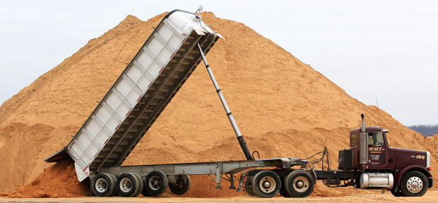 Before beginning this lab, I completed some background reading to inform myself on the effects of fracking truck transportation upon local communities by reading the white paper "Transportation Impacts of Frac Sand Mining in the MAFC Region: Chippewa County Case Study." As the text explains, frac sand mines are often located in remote areas in the country, which means that many of the resources used for the mining process (water, sand, chemicals, drilling equipment) need to be transported to and from the mining site. This transportation has adverse effects upon local roads, which has caused local governments to explore ways to mitigate this damage. Chippewa County, for example, has developed a series of road upgrade maintenance agreements (RUMA) to deal with recovering road damages, funding maintenance, and grading cross improvements (Figure 1).


