GIS II Lab 2: Data Downloading, Interoperability, and Working with Projections in Python

Goals & Objectives

This lab concerned locating, downloading and organizing spatial data.  The study area was Trempealeau County, WI, which pertains to our semester-long GIS II project regarding frack sand mining.  

Specific goals addressed in this lab include increasing proficiency in: 

• downloading data from the internet
• data organization
• importing data to ArcGIS
• joining data
• projecting data from different sources into one coordinate system
• building and designing a geodatabase
• basic Python scripting
• determining data accuracy

Methods

The first section of this lab dealt with data management.  First, I downloaded data about Trempealeau County from six different online sources using the workflow depicted in Figure 1. 

Figure 1: work flow of data management

These sources included:

1. US Department of Transportation
2. USGS National Map Viewer
3. Multi-Resolution Land Characteristic Consortium
4. USDA Geospatial Data Gateway
5. Trempealeau County Land Records
6. USDA NRCS Web Soil Survey

After the data was appropriately downloaded, unzipped, and organized in my personal class folder, I wrote a Python script that clipped and projected the data (displayed in my Python Scripts blog post on this blog).  Then, I utilized ArcGIS to create a cartographically pleasing map displaying the topography of Trempealeau County (Figure 2).  

Next, I examined each dataset's metadata to collect information about scale, effective resolution, minimum mapping unit, planimetric coordinate accuracy, lineage, temporal accuracy, and attribute accuracy.  I recorded all of this information in a table (Figure 3).  

Figure 2: maps of data gathered from USDA Geospatial Gateway, USGS National Map Viewer, Trempealeau County Land Records Division, USDA NRCS Web Soil Survey

Data Accuracy

Figure 3: table depicting data accuracy information about downloaded datasets

Conclusions

After searching the metadata for all of the sources, I found out that much of it was incomplete.  Some sources were better at providing metadata and data accuracy information than others.  When downloading datasets from the internet, it is important to make note of metadata and data accuracy information so you can better analyze your data. 

When using these datasets later this semester for our frack sand mining project, we should keep in mind that our data accuracy information was lacking.  In fact, none of our datasets included information about planimetric coordinate accuracy and only two mentioned the attribute accuracy.  

GIS II: Python Scripts

This blog post will feature all of the scripts that I create during GIS II in Spring 2016.

Python Script 1:

Figure 1: python script used to project rasters

Python Script 2:

In Exercise #7, we wrote a Python script to select the frac sand mines that were:

• active
• not within 1.5 kilometers of a railroad
• without a rail loading station

Figure 2: python script used to select mines 

Python Script 3:

In Exercise #8, we wrote a Python script to create a weighted index risk model for mining locations:

Figure 3: python script used to create risk model

GIS II Lab 1: Frac Sand Mining in WI

Fracking: What is it?

Frac sand mining refers to the process of extracting quartz sand (also known as silica sand) for various uses including paving roads, glass manufacturing, and filtering drinking water.  In order to be of use, this quartz sand must be well-rounded, extremely hard, and uniform in size.  After finding a suitable mining site, excavation, blasting, crushing occur to retrieve the sand, which is then processed.  Following this, the sand must be transported and the mining site must undergo a reclamation process.  

Though fracking has existed for hundreds of years, more attention has surrounded the topic in recent years due to increasing use of quartz sand in the petroleum industry.  This has been particularly apparent in the states in which frac sand mining is occurring, including Wisconsin.  Accessible frac sand is primarily found in western and central Wisconsin (see Figure 1).  

Figure 1: map detailing frac sand mines and sandstone locations in WI

Impacts of Fracking

Although frac sand mining is beneficial for many industries, there are also concerns surrounding the practice and its effects upon the environment and its inhabitants.  Firstly, sand mining facilities negatively impact air quality due to emission of both dust and pollutants as a result of mining processes and equipment.  For example, the loading and unloading of sand poses a threat for dust emissions, while the electrical generators often used at mining operations are release pollutants into the air.  The Wisconsin DNR (WDNR) enforces a variety of regulations regarding air quality standards to ensure safety, however, the risk of reduced air quality is very real.  

Additionally, frac sand mining can have negative impacts upon water resources.  If a site is in close proximity to a river, stream, or wetland, groundwater may be encountered during the excavation process.  This groundwater is often used for washing, cleaning, and sorting materials as well as in facility buildings.  This use must be closely monitored, as the potential for affecting surrounding streams, trout waters, nearby private wells or other water resources exists.  

Furthermore, frac sand mining operations pose a problem for recreational activities such as hunting, trapping, fishing or hiking.  The noise, dust, traffic, lighting, forest loss, and reduced air quality often associated with fracking operations are undesirable to many people who wish to enjoy outdoor activities.    

Fracking in the News

As a result of improved technologies and new developments in directional boring, frac sand mining has become more affordable while previously inaccessible silica sand is now accessible.  Combined with the demand for silica sand for the petroleum industry (among other industries), the fracking industries have taken off in Wisconsin over the past years.  Increasing amounts of mining sites have brought jobs and money to many communities, some of which desperately needed the financial boost.  

However, as Pamela King writes in her Midwest Energy News article, some frac sand mining towns are worried that the fracking boom is peaking and may soon come to an end.  In July 2015, there were 58 inactive extraction sites in WI, with the number of active mining sites sitting barely above this total at 63.  While sand frac mines have caused plenty of controversy regarding topics such as air quality or noise, the mines have also revitalized and enriched communities.  Residents of Chippewa Falls noted that the money stemming from frac sand mining has made a number of new buildings possible in their downtown district, as well as provided employment for community members.  While the fate of fracking remains yet to be seen, King remarks that western Wisconsin's economic diversity could be advantageous in the possible move away from frac sand mining--there are plenty of other industries that contribute considerably to Wisconsin's economy.

GIS + Fracking

GIS technologies can be used to assess and analyze the situations surrounding frac sand mining in Wisconsin.   Frac sand mining requires transportation of materials both to and from processing facilities as well as to other destinations, all of which take a toll on roads.  As a part of this course, we will be using GIS to examine the effects of frac sand transportation upon road quality.  

Sources

King, Pamela. (2015). Wisconsin Towns Worry Frac Sand Boom Will Dry Up. Midwest Energy News. Retreived from http://midwestenergynews.com/2015/06/03/wisconsin-towns-worry-frac-sand-boom-will-dry-up/. 

Wisconsin Department of Natural Resources. (2015). Industrial Sand Mining. Retrieved from http://dnr.wi.gov/topic/Mines/Sand.html.

Wisconsin Department of Natural Resources. (2012). Silica Sand Mining in Wisconsin. Retrieved from http://dnr.wi.gov/topic/Mines/documents/SilicaSandMiningFinal.pdf. 

Wisconsin Geological and Natural History Survey. (2012). Frac Sand in Wisconsin Factsheet. Retrieved from http://wcwrpc.org/frac-sand-factsheet.pdf. 

GIS I Lab 4: Best Location to Live in Boulder County, CO

Introduction: 

My research question for this lab was: Where would be the best place for me to live in Boulder County, Colorado?  My specifics objectives were determining a location to live that would be in a city of less than 50,000 inhabitants, within 1 mile of a water body, within 2 miles of a park, and at least 500 meters away from a major road.  The intended audience is anyone looking for a quieter place to live in a smaller city with access to nature in Colorado.  

Data Sources: 

To answer my research question, I utilized the standard ESRI 2013 data, which was accessible through the university Geography departmental server.  Data concerns included the fact that all data was from 2013, and thus not completely up to date.  In the past few years, Colorado has become an increasingly attractive destination to live, so I would expect the population data might have increased.  Additionally, my cities feature class did not contain every city and town that exists in Boulder County, and some data within it displayed negative numbers or simply stated 'no data.'  

Methods:

Objective 1: Identify Best Location
To ascertain the best location for me to live within Boulder County, Colorado, I first created a file geodatabase and then utilized the university Geography departmental server to export ESRI 2013 data regarding cities, water bodies, parks, and major roads into it.  I then projected my data frame to NAD_1983_StatePlane_Colorado_North, which best fit the location of Boulder County in northern Colorado.  Then, I utilized the Query, Buffer, Intersect, tools to find narrow down my locations to cities with a population under 50,000, within 1 mile of a water body, and within 2 miles of a park.  This left me with three cities.  After this, I utilized the Erase tool to narrow down my locations to cities at least 500 meters from a major road.  This left me with only one city that met all of my parameters, namely Eldora, Colorado.  

Objective 2: Create Map
After completing the analysis portion of the lab, I added a title, legend, scale bar, and compass to my map.  To make my map cartographically pleasing, I picked out an appropriate color scheme and carefully arranged my map elements. To give map readers some perspective, I decided to also  include a locator map displaying the location of Boulder County within Colorado. 

Results:

The results of my methods are displayed below.  After completing my analysis, I found out that only one town (of the cities included in the ESRI 2013 census data) fit all of my parameters: Eldora, Colorado.  

Figure 1: Data Flow Model

Figure 2: Final Map

Evaluation:

Overall, I really enjoyed working on this project.  Unlike with previous labs, this project gave me the opportunity to pick and analyze a topic that I was interested in.  It was very rewarding to see that I could effectively use all of the knowledge and tools that I have learned in GIS I to answer my research question without the guidance of a step-by-step lab guide.  

If I were to do this project again, I would take care to create my file geodatabase right away--during this project, I forgot to create it at the beginning of my work and had to backtrack and export all of my files after I had done the first few steps.  Though most of the project went smoothly, I encountered a few challenges when gathering my data.  When exporting my data, I first used a city feature class that only included a handful of cities; since this seemed problematic to me, I dug around in the ESRI 2013 data for a while before finding out that there was a "detailed" city feature class that included 22 cities for Boulder County.  

GIS I Lab 3: Vector Analysis

Introduction: 

The purpose of this lab is to utilize various geoprocessing tools for vector analysis in ArcGIS to determine a suitable habitat for bears in the study area of Marquette County, Michigan.  

Methods:

Objective 1: Map Black Bear Locations

To achieve this objective, I first opened ArcCatalog, navigated to my personal Lab 3 folder and examined the data stored there, taking note of the data's coordinate system.  Then, I used the search function in ArcHelp to read more about adding x,y coordinate data as a layer.  To add the bear locations as an XY event theme, I navigated to File, Add Data, and Add XY Data, filling out the pop up window with appropriate information.  This included choosing "bear_locations_geo$" as the table as well as choosing the correct coordinate system, NAD_1983_HARN_Michigan_GeoRef_Meters.  

Objective 2: Determine Forest Types
To achieve this objective, I added all of the feature classes from the bear_management_area data set to a data frame.  I then changed the symbology of the landcover feature class to "unique values" based off of the MINOR_TYPE value field, choosing an appropriate color scheme.  In order to determine the bear habitat, I performed a Spatial Join between the bears_locations and landcover feature classes to generate a new feature class which displays both the ID number of the bear and the land cover type in which it was found in the attribute table.  After this, I used the Summarize tool on the MINOR_TYPE field to generate a table displayed the number of bears found in each type of habitat.  The top three habitat types were Mixed Forest Land, Forested Wetlands, and Evergreen Forest Land.  

Objective 3: Examine Black Bears & Streams
To achieve this objective, I utilized Select By Location to discover how many bears were found within 500 meters of a stream.  Upon doing this, I found out that 72% of bears were found near streams, thus making this an important criterion in determining suitable bear habitats.  I then performed a Buffer on the streams layer to create a buffer of 500 meters around the streams feature class. 

Objective 4: Determine Suitable Black Bear Habitat Regarding Streams & Landcover
To achieve this objective, I first performed a Query upon the landcover feature class to select the top three habitat types and created a separate feature class from this selection.  Then, I performed an Intersect using that landcover_top3 feature class and the streams500 feature class created in Objective 3.  I then used the Dissolve tool to remove the internal boundaries.  

Objective 5: Determine Suitable Black Bear Habitat in Michigan DNR Areas
To achieve this objective, I first added the dnr_mgmt feature class to my ArcMap document.  Since this feature class included superfluous information about DNR areas in all of Marquette County, I performed a Clip using the study_area feature class to create a feature class showing only the DNR areas within the study area.  Then, I performed a Dissolve upon the newly created feature class to remove the internal boundaries.  After this, I used the Intersect tool on the dnr_mgmt and landcover_top3 feature classes.

Objective 6: Eliminate Unsuitable Areas
To achieve this objective, I first performed a Query on the landcover feature class to select all of the Urban or Built Up land, creating a separate feature class entitled urbanland from this selection.  Then, I used the Dissolve tool to remove the internal boundaries.  After this, I performed a Buffer of 5 kilometers on the urbanland feature class.  Then, I utilized the Erase tool, using dnr_mgmt as the input and urbanland as the erase feature to create the output feature class final_hab, which displays the suitable areas for bear habitats.  

Objective 7: Create Map & Data Flow Model

To achieve this objective, I created a cartographically pleasing map that displayed suitable areas for bear habitats.  After this, I created a data flow model depicting the steps I used during this lab.  Both the map and data flow model are displayed below in the Results section.  

Objective 8: Python Application

Figure 1: Python Commands

To achieve this objective, I utilized Python in ArcMap to write buffer, intersect, and erase commands using the bear habitat data.  

Results:

Figure 2: Data Flow Model

Figure 3: Final Map

The results of my methods are displayed above.  

Sources:

Center for Shared Solutions and Technology Partnerships. (2014). Michigan Geographic Framework: Marquette County. Retrieved from http://www.mcgi.state.mi.us/mgdl/framework/metadata/Marquette.html.

Michigan Center for Geographic Information. (2002). Michigan 1992 NLCD Shapefile by County. Retrieved from http://www.mcgi.state.mi.us/mgdl/nlcd/metadata/nlcdshp.html. 

Michigan Department of Natural Resources. (2001). Wildlife Management Units. Retrieved from http://www.mcgi.state.mi.us/mgdl/nlcd/metadata/nlcdshp.html.

State of Michigan. (2015). GIS Open Data. Retrieved from  http://gis.michigan.opendata.arcgis.com/

GIS I Lab 2: Downloading GIS Data

Introduction: 

The purpose of this lab is to learn how to download and map data from the US Census Bureau.   

Methods:

Objective 1: Download 2010 Census Data

To achieve this objective, I navigated to the US Census Bureau Fact Finder Website and utilized the Advanced Search function.  Under the Topics option, I chose "People, Basic Count/Estimate" and then "Population Total."  Under the Geography option, I chose "County 050," "Wisconsin," and "All Counties in Wisconsin."  Then, I scrolled through the provided data and located the variable P1 for Total Population from the 2010 SF1 Dataset.  I downloaded this file to my personal Lab 2 folder, extracting all files from the provided zip file.  

Objective 2: Download Shapefile of 2010 Census Boundaries

To achieve this objective, I navigated once more to the US Census Bureau Fact Finder Website and utilized the Advanced Search function again.  Under the Geographies option, I selected the Map tab, noting that the Wisconsin counties were highlighted.  I then downloaded this information to my personal Lab 2 folder, extracting all files from the provided zip file.  

Objective 3: Join Downloaded Data to Census Shapefile

To achieve this objective, I first opened up a blank map in ArcMap, being sure to save the file to my personal Lab 2 folder.  Then, I renamed the Layers data frame as "Population" and added the 05_00 shapefile (acquired in Objective 2) and the P1 table (acquired in Objective 1) to the map.  After this, I joined the two data files through clicking on the shapefile, selecting "Joins and Relates" and then "Join."  Upon opening the shapefile's attribute table, the joined data is visible in the last column entitled D001, which contains population data. 

Objective 4: Mapping Data
To achieve this objective, I needed to add a new field to the 05_00 shapefile, since the original D001 field was imported as a string field type and could not be mapped quantitatively.  This involved opening the shapefile's attribute table, selecting "Add Field," naming the new file (D001_new), and choosing the field type to be "Double."  Then, I right-clicked the newly added field, opened the Field Calculator, and selected the original D001 field.  After this, I was able to map Wisconsin's population by utilizing the shapefile's "Properties" window to select D001_new in the "Value" field as well as choose an appropriate color ramp and number of classes.  

Objective 5: Mapping Another Variable

To achieve this objective, I returned to the US Census Bureau Fact Finder Website and selected another variable to download, namely Total Housing Units in Wisconsin by County.  I then followed the steps listed above in Objectives 2, 3, and 4 to download, unzip, and add, join, and map the data.  

Objective 6: Configure Map Layout

To achieve this objective, I first changed the projections of both data frames (Population and Housing) to NAD 1983 Wisconsin TM, which is more suitable for the state.  I then inserted a title, legend, scale, north arrow, base map and source for each map.  To make the layout cartographically pleasing, I utilized rulers and grid lines to neatly arrange my map elements.  Finally, I added a neat line around the entire layout.  

Objective 7: Create Webmap

To achieve this objective, I made a copy of my map document, as I wanted to preserve my original maps as well as create a new document displaying just the housing data for a webmap.  I then logged into my ArcGIS Online Account inside ArcMap.  After making necessary adjustments to the new document, I shared and configured my map through creating a web map service on ArcGIS Online.  

Results:

Figure 1: Maps displaying demographic and housing data

Figure 2: Interactive webmap displaying WI housing data;
located on ArcGIS Online here

The results of my methods are displayed above.  Figure 1 depicts both population and housing data; as would be expected, the maps are similar in that in locations where more people are present, there are more houses.   

Sources:

U.S. Department of Commerce. (2015).  American Fact Finder. Retrieved from http://factfinder2.census.gov/faces/nav/jsf/pages/searchresults.xhtml?refresh=t 

GIS I Lab 1: Base Data

Goal and Background: 

The purpose of this lab was to learn about various spatial data sets and how to accurately present them through creating a basic report featuring base maps.  This report concerns the Confluence Project, a new development in downtown Eau Claire, Wisconsin which will serve as a community arts center, university student housing, and a commercial retail complex.  

Methods:

Objective 1: Explore various data sets for the City and County of Eau Claire

To achieve this objective, I used ArcMaps and provided spatial data to become familiar with the Eau Claire Geodatabase.  As a part of this, I explored various feature datasets, feature classes, including data regarding parcels, zoning, topology and census.  

Objective 2: Digitize the site for the proposed Confluence Project
To achieve this objective, I created a new geodatabase in ArcCatalog.  I then added a feature class to this geodatabase, and imported the BlockGroups data from the Eau Claire Geodatabase.  After that, I added the pro_site feature class to the same data frame.  In order to begin the digitizing process, I opened the Editor Toolbar and utilized it to digitize the Confluence Project area.

Objective 3: Learn about the Public Land Survey System

To achieve this objective, I first inserted a new data frame and added a basemap imagery layer.  I then added the PLSS_Townships feature dataset from both of the Eau Claire Geodatabases.  Using the Properties window, I added numbers to the PLSS sections as well as utilized a stretched color scheme to highlight patterns.  I then identified the specific PLSS section in which the Confluence Project was located.  

Objective 4: Create a legal description for parcels and generate basic site report

To achieve this objective, I navigated to the City of Eau Claire's Property Search website.  After zooming in on Eau Claire and locating the two parcels involved in the Confluence Project, I clicked on each of them to collect the information needed to write a proper legal description for the parcels.  I also took a screenshot of each parcel selected and displayed its parcel ID.  The finished product is displayed below.  


Brief legal descriptions for Confluence Project properties' location of site in Public Land Survey System: 

I. PARCEL 1 

Figure 1: Parcel 1

Parcel Number: 02-0365 
PIN: 1822122709200042068
Street Number:  128 
Street Name: Graham Ave. 
Owner's Name: Haymarket Concepts LLC 
Owner's Address: PO Box 617
Owner's City, State, Zip: Eau Claire, WI 54702

Legal Descriptions: LOTS 1-2-3-4-5-6-7-8 BLK 62 & THE 26 FT W OF E 84 FT OF LOTS 9 & 10 & EX E 140 FT ALL OF LOTS 9 & 10 BLK 62 VILLAGE OF EC ADD TID 8


II. PARCEL 2 

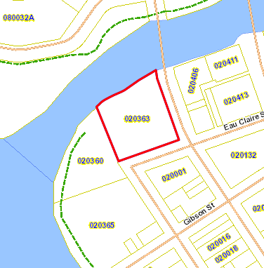
Parcel Number: 02-0363 

Figure 2: Parcel 2

PIN: 1822122709200049005
Street Number: 202 
Street Name: Eau Claire St.
Owner's Name: Haymarket Concepts LLC 
Owner's Address: PO Box 617
Owner's City, State, Zip: Eau Claire, WI 54702

Legal Descriptions: PRT OF BLK 58 IN GOV LOT 4 BEING REPLATTED AS LOT 1 CSM 3037 REC V 17 P 95 DOC 1109271 LOC IN GOV LOT 4 SEC 20-27-9 TID 8 **FOR 2015 COMBINED PARCELS 02-0360-A, 02-0357, 02-0358, 02-0359, 02-0361, 02-0362

Objective 5: Build a layout with each of the major thematic feature classes

To achieve this objective, I created six different basemaps presenting various relevant data about the Confluence Project (Figure 1, below).  The maps addressed Civil Divisions, Census Boundaries, PLSS Features, EC City Parcel Data, Zoning, and Voting Districts.  

Process: To neatly organize my data, I utilized rulers and guidlines to set up six data frames.  I then added basemap imagery data to each data frame, as well as an appropriate title.  Each map required adding different data from the Eau Claire Geodatabases, and then adjusting transparency levels and color schemes to assure a pleasing map.  After the data was in place, I inserted a scale bar (in miles) as well as a legend for each map.  

Results:

The results of my methods are displayed below in the form of six basemaps.  Together they present useful information which could aid developers in decisions concerning the Confluence Project construction.

Figure 3: Finished Project

Sources:

City of Eau Claire, WI (2015).  City of Eau Claire Property Search.  Retrieved from http://eauclairecitywi.wgxtreme.com/ 

Zoning Districts and Maps (2011). Eau Claire.  Retrieved from Q:\StudentCoursework\CHupy\GEOG.335.001.2161\LAB\lab1

Lippel, Irene D. (2000).  Understanding Wisconsin Township, Range and Section Land Descriptions. Geological and Natural Historical Survey.  Retrieved from Q:\StudentCoursework\CHupy\GEOG.335.001.2161\LAB\lab1